Base validation

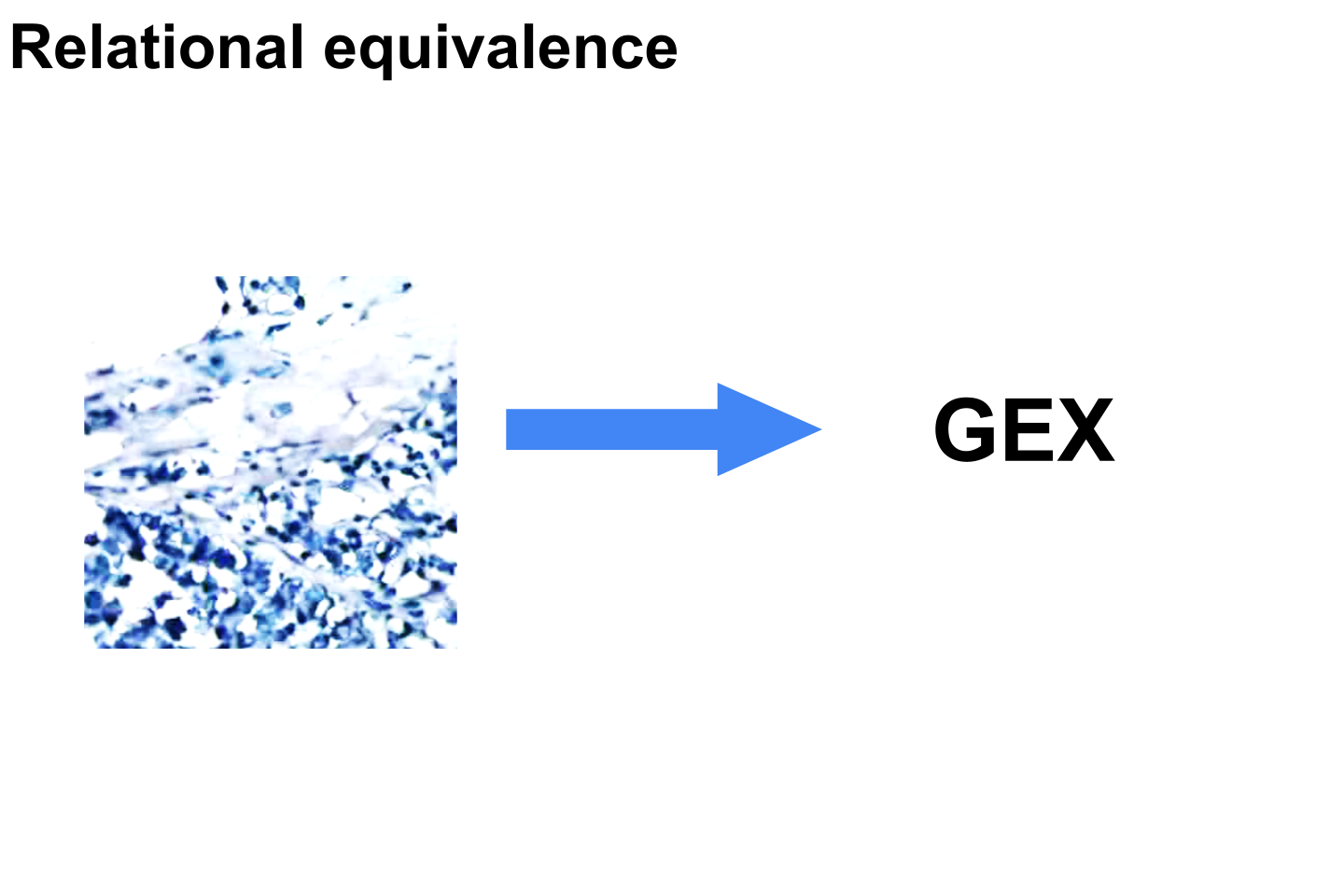
GeneCodeR base validation via relational equivalence

Reload important files recently saved:

main_path <- "~/Documents/main_files/AskExplain/Q4_2022/gcode/"

# Please replace this path
path_to_save <- paste(main_path,"./temp_save_dir/",sep="")

load(file = paste(sep="",path_to_save,"all_genecoder.RData"))

Set up the test configuration for GeneCodeR

# Set up genecoder transform information
genecoder.config <- GeneCodeR::extract_config_framework(F)
genecoder.config$transform$from <- 1
genecoder.config$transform$to <- 2
genecoder.config$extract_spots$window_size <- 30

Set up validation functions to evaluate statistically significant differences via a t-test, and, cosine similarity.

# Testing functions

# cosine metric for similarity between observations

test_sample_and_genes <- function(a,b,non_zero_markers,test_type="cosine"){

  if (test_type == "t.test"){
    
    return(
      list(
        
        sample_wise = do.call('c',parallel::mclapply(c(1:dim(a)[1]),function(X){
          
          t.test(as.numeric(a[X,non_zero_markers[X,]]),as.numeric(b[X,non_zero_markers[X,]]))$p.value
          
        },mc.cores = 8)),
        
        gene_wise = do.call('c',parallel::mclapply(c(1:dim(a)[2]),function(X){
          
          t.test(as.numeric(a[non_zero_markers[,X],X]),as.numeric(b[non_zero_markers[,X],X]))$p.value
          
        },mc.cores = 8))
        
      )
    )
  } 

  if (test_type == "cosine"){
    return(
      list(
        
        sample_wise = do.call('c',parallel::mclapply(c(1:dim(a)[1]),function(X){
          
          lsa::cosine(as.numeric(a[X,non_zero_markers[X,]]),as.numeric(b[X,non_zero_markers[X,]]))
          
        },mc.cores = 8)),
        
        gene_wise = do.call('c',parallel::mclapply(c(1:dim(a)[2]),function(X){
          
          lsa::cosine(as.numeric(a[non_zero_markers[,X],X]),as.numeric(b[non_zero_markers[,X],X]))
          
        },mc.cores = 8))
        
      )
    )
  } 
}

Base validation

Base validation is used to directly compare observed gene expression with transformed image spots representing gene expression via pattern matching and weight assignment. Cosine similarity is used to compare the observed and the transformed.

# Base testing

# Extract test spot data

base_test_spot_data <- GeneCodeR::prepare_spot(file_path_list = test_file_path_list,meta_info_list = meta_info_list,config = genecoder.config, gex_data = test_gex_data$gex)

## [1] "Extracting spots"
## [1] "Preparing spot      1"
## [1] "Preparing spot      2"
## [1] "Preparing spot      3"
## [1] "Preparing spot      4"
## [1] "Preparing spot      5"
## [1] "Preparing spot      6"
## [1] "Preparing spot      7"
## [1] "Done preparation!"

# Important non-zero markers (gene is expressed)
non_zero_markers <- base_test_spot_data$gex>0



base_spot2gex <- GeneCodeR::genecoder(model=genecoder.model, x = base_test_spot_data$spot, config = genecoder.config, model_type = "gcode")
    
base_spot2gex <- test_sample_and_genes(a = base_test_spot_data$gex, b = base_spot2gex,non_zero_markers = non_zero_markers, test_type = "cosine")

save(base_spot2gex,file = paste(sep="",path_to_save,"base_spot2gex.RData"))

load(file = paste(sep="",path_to_save,"base_spot2gex.RData"))

title_name = "base_cosine_similarity"
tissue_name = "breast"

sample_similarity = base_spot2gex$sample_wise
feature_similarity = base_spot2gex$gene_wise

library(ggplot2)

lm <- rbind(c(1,2),
            c(1,2),
            c(1,2))

g1 <- ggplot(data.frame(Measure=sample_similarity,Metric="Predicted vs Observed \n Sample-wise Pearson Correlation"), aes(x=Metric,y=Measure)) + 
  geom_violin() + ylim(-1,1) 

g2 <- ggplot(data.frame(Measure=feature_similarity,Metric="Predicted vs Observed \n Gene-wise Pearson Correlation"), aes(x=Metric,y=Measure)) + 
  geom_violin() + ylim(-1,1) 

gg_plots <- list(g1,g2)

library(grid)
library(gridExtra)
final_plots <- arrangeGrob(
  grobs = gg_plots,
  layout_matrix = lm
)

plot(final_plots)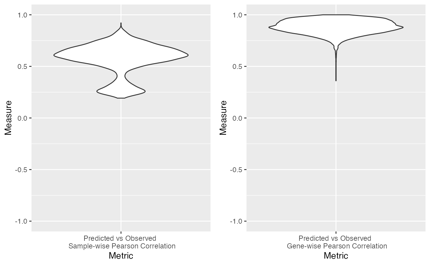

ggsave(final_plots,filename = paste(path_to_save,"/jpeg_accuracy_gcode_",tissue_name,"_SPATIAL/",title_name,"_accuracy_",tissue_name,"_spatial.png",sep=""),width = 5,height=5)


rm(list=ls())
gc()

##           used (Mb) gc trigger    (Mb) limit (Mb)   max used    (Mb)
## Ncells 1141178 61.0    2946211   157.4         NA    2946211   157.4
## Vcells 2072506 15.9 1535690653 11716.4      16384 1382898229 10550.7

help@askexplain.com

2022-12-18

GeneCodeR base validation via relational equivalence